AIM-UC
Program for Electronic Charge Density Analysis: User Manual


Table of Contents


1 Introduction to AIM-UC


1.1 About del program

The AIM-UC program generates some graphics related to Atoms in Molecules theory (AIM) developed by Richard Bader. The data input of the program is a 3D electronic charge density grid. This program is able to find the critical points of electronic charge density and positioning a plane in the 3D grid space to calculate graphics of charge density, negative Laplacian, contour maps, gradient fields, molecular graph and basin bounds. It was programmed completely in C / C++ language, using FLTK 1.x.x (a GUI toolkit) and OpenGl 1.3, as external libraries. The program was developed in the Laboratorio de Química Computacional, Facultad de Ciencias y Tecnología (FACYT), Universidad de Carabobo, Venezuela. It was funded through the FONACIT project number G-2005000424.

Please cite this paper: D. Vega and D. Almeida, Journal of Computational Methods in Science and Engineering 14 (2014), 131-136. ➤➤➤

Authors:
David Vega M. Alternate email address: dvega68@yahoo.com
Daniel Almeida


1.2 Minimum system requirements

The current version of AIM-UC program requires:
Operative System: Windows, Ubuntu, Xubuntu and Centos.
System memory: 500 MB
Graphic card: 128 MB


1.3 Installation

Download the aim-uc.v1.3.7z (Win32) or aim-uc64.v1.3.7z (Win64) file and expand it to an empty folder. In this folder, if desired, create another folder called “manual” and decompress the manual_aimuc_en.7z file within.
Now available for Linux: Ubuntu 12.10, Xubuntu 12.10 and Centos 6.3.

NOTE: All files are compressed in 7zip format.


1.4 License

Feel free to use and distribute this program.

There is no warranty for the program, to the extent permitted by applicable law. The program is provided “as is” without warranty of any kind, either expressed or implied, including, but not limited to, the implied warranties of merchantability and fitness for a particular purpose.

[Table of Contents]


2 Loading data


2.1 Loading a grid file

In the main menu, click “File” option and then click “Open File” option.

MENU FILE
A file browser appears allowing to select the file that contains the grid or wavefunction data. In this AIM-UC version, any of the following file formats can be selected:

Dmol grid data: File *.grd from Dmol3
Gaussian cube: File cube from Gaussian
Gamess cube: File *.dat from Gamess that contains one or more grids
VASP CHGCAR: File CHGCAR from VASP
AIMPAC wavefunction: File *.wfn from AIMPAC
binary data: File that contains grids in binary format
OPEN FILE

Then find the file in the appropriate directory, select it and press the “OK” button. If the current file does not contain the atom coordinates, it is necessary loading them from another file. The accepted file formats are *.car, *.mol and *.xyz.

After the file is loaded, the grid limit box and a plane will appear. The plane will be in a default position (In the case of *.wfn files, to maintain compatibility with containing grid files, also a box is drawn).


2.2 Modifying the plane position

After load the file that contains the grid data and the one that contains the atom coordinates, the default plane position can be modified by clicking on the menu “Edit” option and then clicking on the “Plane Position” option.

MENU EDIT

The x, y, z coordinates of the origin point and the two defining plane vectors can be modified in the “Vector Positions” section of the appearing window. One of 9 different default positions can be selected in the “Default Positions” section

PLANE TOOLS

The window shows the plane “Rotation” and “Translation” options by using as axes (direction, in translation case) the normal vector of the plane and parallel vectors to the two plane defining vectors. The rotation “Angle” (expressed in degrees) and the translation distance (Step) can be modified. It is possible to change the plane dimensions (Size) and also the angle between the vectors that define the plane (Shape), so the angle could be different from 90°. The “Plane from selected” section permits to build a plane that contains three selected elements (to select click on the atoms or critical points with the mouse left button). The “Selection mode” checkbox must be marked.


2.3 Creating the plane grid

After positioning the plane, a 2D grid, used to calculate contour maps, critical points in the plane, gradient field, molecular graph and atomic basin bound, can be created.

Click the “Process” option and then click the “Create Plane Grid” option.

MENU PROCESS

A window appears, and once the numbers of 2D grid intervals are introduced, click “Accept” button.

CREATE PLANE

The charge density and the negative laplacian planes (with the same dimensions) will be built.

[Table of Contents]


3 2D Visualization


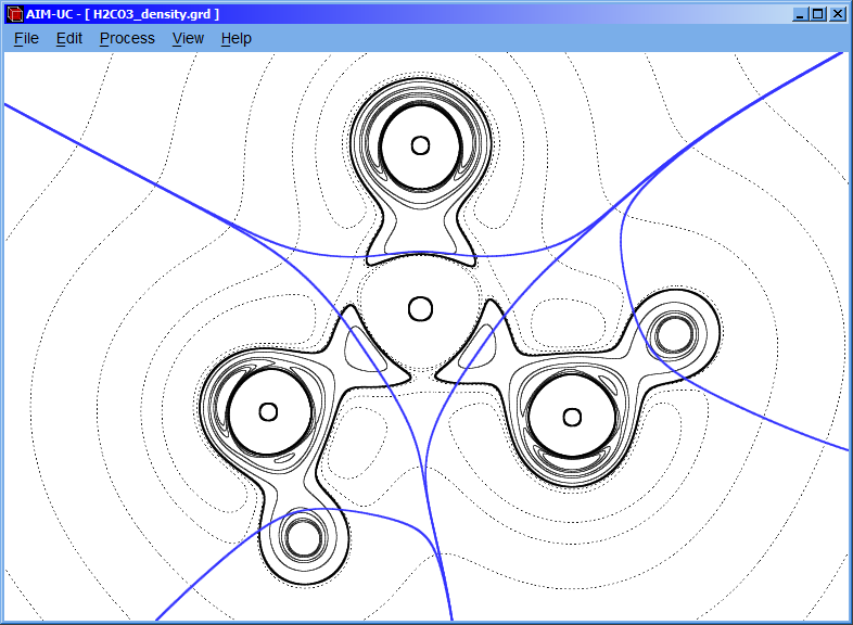
3.1 Calculating contour map

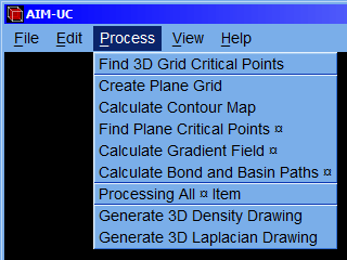
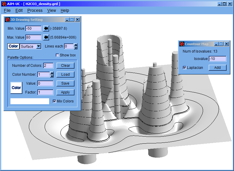
Click the “Process” option and then click the “Calculate Contour Map” option.

Following, a setting window will appear and introduce the isovalues of charge density. Then click the “add” button; if “Laplacian” checkbox is marked, then it will calculate the contour of the negative laplacian, instead of the contour of the charge density.

CONTOUR MAP

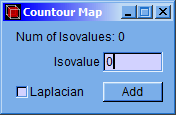
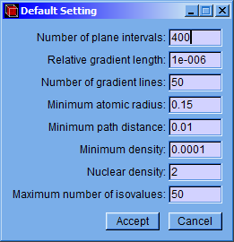
NOTE: The maximum number of isovalues that can be added is 50. This number can be modified in the “Default Settings” window, explained in section 5.

For viewing the contour map, click the “View” option and then click the “Change Display” option.

CHANGE DISPLAY

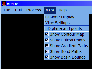
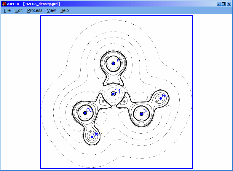
The contour line corresponding to the added isovalue can be visualized in this way.

EXAMPLE CONTOUR

NOTE: If the plane dimensions or positions are changed, it is necessary to create again the plane and recalculate the contour map.


3.2 Finding plane critical points

The program finds the critical points in the 3D space contained by limit box and the charge density plane.

For calculating the critical points in the 3D grid, click the “Process” option and then click the “Find 3D Grid Critical Points” option. The critical points on the plane can be calculated by clicking the “Process” and the “Find Plane Critical Points” options.

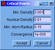
After that, a setting window (Critical Points) will appear allowing to modify minimum density, nuclear density, minimum atomic radius and convergence factor values. Although the program has default values, they can be easily changed in this window. Then click the “Accept” button to find the critical points.

CRITICAL POINTS

Min. Density: Minimum value of the electronic charge density. A critical point with charge density below this value will not be stored.
Nuclear Density: Value of the electronic charge density; the search of maximum critical points will start up to this value. The high electronic charge density around the atom nuclei makes the gradient module increases too fast, under such a condition the Newton-Raphson method fails. Due to this fact a simple searching method is used for those points of the grid that have a charge density above the “Nuclear Density” value.
Min. Atom Radius: If the distance from an atom nucleus to a critical point is lower than this value, then the critical point will not be stored. This prevents fake critical points originated by the oscillation of the interpolation polynomial near the atom nuclei.
Convergence: Criterion applied to the gradient that allows deciding whether it is a critical point. In order to consider it as a critical point, the module of the gradient vector divided by the charge density, all this multiplied by itself must be lower than the Convergence value.

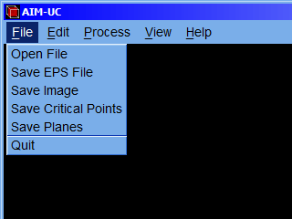
Information of the 3D critical points could be saved in a file. Click the “File” option followed by the “Save Critical Points” option.

NOTE: In the case of search of critical points (3D) in *.wfn files, the “Nuclear Density” value is not used. The searches start at the midpoints of every pair, trio and quartet of atoms.


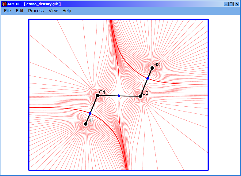
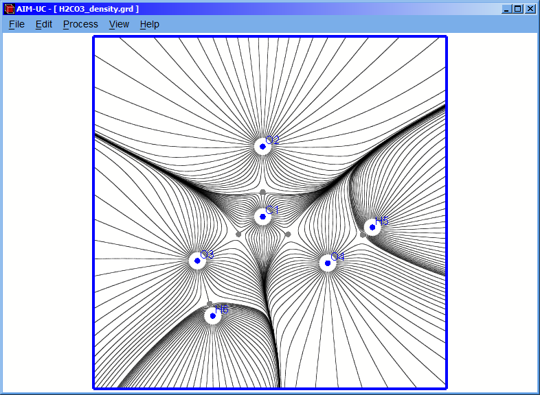
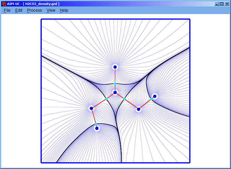
3.3 Calculating gradient field

Click the “Process” option and then the “Calculate Gradient Field” option.

NOTE: Plane critical points must be calculated before doing the gradient field calculation.

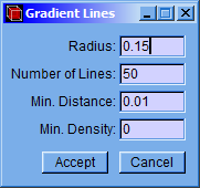
A setting window (Gradient Lines) will appear in which the values of the radius, number of gradient lines and the minimum distance can be set. Although the program has default values, they can be easily changed in this window. Then click “Accept” button to calculate the gradient field.

GRADIENT LINES

Radius: Distance from the nucleus to the beginning point of the gradient lines.
Number of lines: Amount of gradient lines that will be shown around each atom.
Min. Distance: Minimum distance between two consecutive points of the gradient path (The fourth order Runge-Kutta method is used, and the path follows the negative gradient).
Min. Density: The electronic charge density is evaluated in each point of the gradient path; the calculation of the current path stops if it is less than the “Min. Density” value.
EXAMPLE GRADIENT

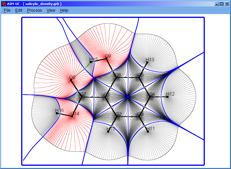
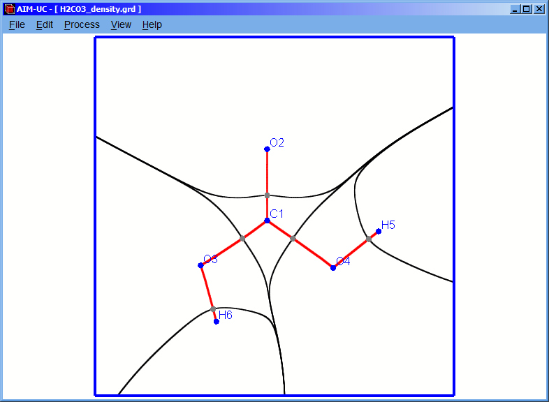
3.4 Calculating bond and basin paths

Click the “Process” option and then the “Calculate Bond and Basin Paths” option.

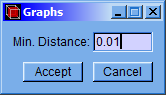
A setting window will appear in which the minimum distance value can be modified, then click the “Accept” button.

GRAPHS

NOTE: Before calculating the bond and basin paths, the plane critical points must be found.

NOTE: It is also recommendable to calculate the 3D critical points (explained in section 3.2) to correct the molecular graph, hiding the paths that do not represent any bond.

EXAMPLE GRAPHS

3.5 Processing all ¤ items

By clicking on an option it is possible to calculate the plane grid (if it was not calculated), the critical points, the gradient field, the molecular graph and the interatomic basin bounds. For this, click menu “Process” option and then the “Processing all ¤ item” option, after a few seconds an information window will appear indicating that all those items were successfully calculated.

EXAMPLE ALL

3.6 2D Drawing settings

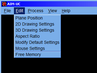
Click the menu “Edit” option and then the “2D Drawing Settings” option.

A setting window with tabs will appear allowing modify some characteristics of the drawing.

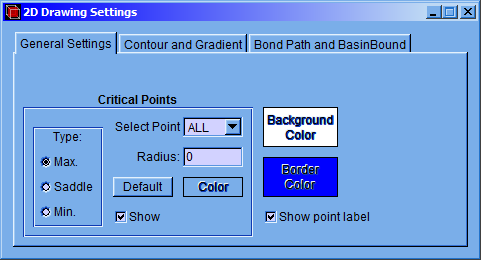
3.6.1 General settings

In the “General Settings” tab of the “2D Drawing Settings” window the “Background Color” and the “Border Color” can be selected. The “Show point label” checkbox will show the critical point tags; the “Radius” and “Color” of the different critical points on the plane: maximum (Max.), minimum (Min.) and saddle points (Saddle) can be modified. Besides, the “Show” checkbox allows whether a critical point will be shown.

2D GENERAL SETTINGS

3.6.2 Modifying contour map and gradient lines

In the “Contour and Gradient” tab some characteristics of the contour map and the gradient field can be modified.

2D CONTOUR SETTINGS

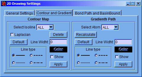
On the left side of the window, the “Contour Map” section, the type, color, and width of the line can be changed and deciding whether the line is shown. These modifications can be applied to individual isoline (selecting just one isovalue in “Select Isoline”) or to the group (selecting “ALL”). The characteristics of the lines can be turned back to their defaults by pressing the “Default” button.

After modify the characteristics, click the “Apply” button to enter the changes.

NOTE: When the “Laplacian” checkbox is activated, the characteristics of the negative laplacian contour map (instead of the density contour map) will be modified.

On the right side of the window, the “Gradient Path” section, the characteristics of the gradient field lines that belong to any atom can be modified. Clicking the “Select Atom” menu the gradient lines of a specific atom or all of them can be modified. Click the “Apply” button to enter the changes.

By clicking the “Recalculate” button, it is possible to change all the options explained in section 3.3, for a single atom or all of them.

3.6.3 Modifying molecular graph and interatomic basin bounds

In the “Bond Path and BasinBound” tab the characteristics of the molecular graph and interatomic basin bounds can be modified.

2D GRAPH SETTINGS

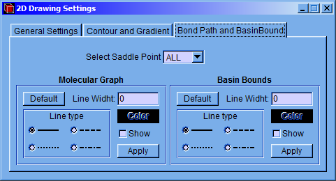
On the left side of the window, “Molecular Graph” section, the type, color, and width of the line can be set and deciding whether the line is shown. On the right side, “Basin Bounds” section, it is possible to do the above indicated changes with the lines of the interatomic basin bound. These modifications can be applied to individual or group by selecting a single saddle point or all of them in the “Select Saddle Point” menu. The characteristics of the lines can be turned back to their defaults by pressing the “Default” button.

[Table of Contents]


4 3D Visualization


4.1 3D Density Drawing

Click the “Process” menu and then the “Generate 3D Density Drawing” option.

After a few seconds the 3D graphic of the electronic charge density will appear.

EXAMPLE 3D DENSITY

Click the “Edit” menu option and then the “3D Drawing Settings” option.

3D SETTINGS

A setting window will appear and it is possible to modify the minimum and maximum values of density, the background and surface color and the line of the drawing. The distances among surface lines can be set by changing the “Lines each” value (for value 0, lines are not shown).

NOTE: If the 2D contour map has already been created (see section 3.1), the contour map isolines will appear on the surface when the “Show Contour Map” checkbox at the menu “View” option is marked.

EXAMPLE 3D DENSITY
In “Palette Options” section, a palette for coloring the drawing according to the density value (z axis) can be created or loaded from a file:

Number of Colors: Number of colors in the palette (maximum 32).
Color Number: Color position in the palette.
Value: Density value corresponding to the color position.
Color: button for changing the color.
Factor: Value by which the charge density is multiplied before being assigned a color from the palette.
Clear: Deleting colors and values of the palette.
Load: Loading the palette from a file (a simple text file with .rgb extension).
Save: Saving the palette.
Apply: Coloring the drawing.
Mix Colors: Colors will be mixed to make a continuous transition between them.

The palette is shown at the left bottom of the window.

EXAMPLE 3D DENSITY

4.2 3D Laplacian Drawing

Click the menu “Process” option and then the “Generate 3D Laplacian Drawing” option. To edit the drawing click the menu “Edit” option and then the “3D Drawing Settings” option. The options for the electronic charge density drawing explained in section 4.1, are the same for this drawing.

EXAMPLE 3D LAPLACIAN

[Table of Contents]


5 Modifying default settings

Click the menu “Edit” option and then the “Modify Default Settings” option.

MENU EDIT

A setting window will appear and in which the default values of the program can be modified.

DEFAULT SETTINGS

The values capable to be modified are: the number of plane intervals, relative gradient length, number of gradient lines, minimum atomic radius, minimum path distance, minimum density, nuclear density and maximum number of isovalues.

[Table of Contents]


6 Mouse settings

The 2D and 3D drawings can be moved or scaled with the mouse; in addition, the 3D drawing can also be rotated.

The action for each mouse button can be set, for this, click the menu “Edit” option and then the “Mouse Settings” option.

MOUSE SETTINGS

On the appearing windows (mouse button) select any of the option buttons (left, middle or right), then choose an “Action” (move, size or rotate) by clicking the drop-down list.

NOTE: If the selected action is already assigned to another button, the action of the first button will be erased.

Move the drawing:
Put the cursor on the drawing and press and hold the assigned mouse button to “move” action and then drag the drawing to the desired position.

Resize the drawing:
Put the cursor on the drawing and press and hold the assigned mouse button to “size” action and then drag the mouse up to increase the drawing dimensions or drag it down to decrease.

Rotate the drawing:
Put the cursor on the drawing and press and hold the assigned mouse button to “rotate” action and then drag the mouse in some direction to rotate the drawing. This option is unavailable for 2D drawings.

[Table of Contents]


7 Drawing views


7.1 Change display

If the drawings in 2D and 3D have been created before, the view among both and 3D grid boundary (with the plane and atoms) drawing can be toggled by clicking the menu “View” and “Change Display” options.


7.2 View settings

Click the menu “View” option and then click the “View Settings” option.

VIEW SETTINGS

The Reflect and Rotate options have the same effect on all drawings and they can be used to invert 2D drawings. The “Reset view” button restores the default view of drawing. The “Z scale” value affects only graphics of electron charge density and its negative Laplacian.

The lighting of the 3D drawing can also be changed. The roller controls (vertical and horizontal) move the position of the light focus, meanwhile “Shininess” y “Specular” slider controls set the shine and the reflection of light on the surfaces. By unmarking the “Enable lighting” checkbox, the light effects will be disabled.

To create a colored contour map of charge density or negative laplacian, the corresponding 3D surface should be generated and colored according to section 4.1. Finally unmark the “Enable lighting” checkbox and click the “Reset view” button.

EXAMPLE LAPLACIAN

7.3 3D view settings of plane, atoms and critical points

Click the menu “View” option, and then the “3D plane and points” option.

VIEW 3D PLANE AND POINTS

A setting window will appear. Click on the “atoms” checkbox to decide whether the atoms are shown. The same can do it with the different types of critical points: Bonds, Rings and Cages.

The “Show point label” checkbox allows whether the tags of the critical points will be shown. The “Resolution” and the “Scale” of the spheres that represents the atoms and critical points can be changed. The resolution value goes from 1 to 100.

Besides, the “Show plane” checkbox allows whether the plane will be shown, and its color can be changed by clicking the “Color” button.

NOTE: The changes on the resolution and scale of the spheres and the plane color are permanent.

EXAMPLE 3D POINTS

NOTE: AIM-UC generates an “aim-uc.dat” file containing the color of the atoms, taken from Jmol program and the atomic radius in Angstroms, taken from the “element.txt” file from the source code of the Open Babel program. These values can be changed in the file. By deleting this file, the default settings will be restored.


7.4 Hide drawing items

Click the menu “View” option and unmark the checkbox to hide any of drawing items: the contour map, critical points, gradient field, molecular graph and interatomic basin bounds.

Show Contour Map: Shows contour maps, the charge density and the laplacian, in 2D and 3D drawings.
Show Critical Points: Shows the critical points on 2D drawing.
Show Gradient Path: Shows the gradient field on 2D drawing.
Show Bond Paths: Shows molecular graph on 2D drawing.
Show Basin Bounds: Shows interatomic basin bounds on 2D drawing.

NOTE: These options do not affect the EPS drawings.

[Table of Contents]


8 Saving a 2D drawing in EPS format

To save an image of the 2D drawing, click the menu “File” option and then the “Save EPS File” option.

Then a window will appear allowing to select the directory where the image will be saved. Enter the name of the image file and click “Save” button.

NOTE: In the EPS drawing will appear those items calculated for 2D drawing (the contour map, the critical points, the gradient field, the molecular graph and the interatomic basin bounds). To learn how to hide some of the items in the drawing, see section 3.6.

[Table of Contents]


9 Saving a drawing screenshot

Click the menu “File” option and then the “Save Image” option to take a screenshot and save it with PNG or BMP format. A window will appear allowing to select the directory where the image will be saved. Select the image type, enter the name of the image and click “Save” button.

[Table of Contents]


10 Some program screenshots


10.1 Positioning the plane through three atoms of ethane

The ethane grid was loaded, and the “Show point label” and “Selection mode” checkboxes were marked, then the atoms C1, C2 y H3 were selected (in yellow):

EXAMPLE ETHANE

The “Make Plane” button was clicked to make a plane through the three atoms:

EXAMPLE ETHANE 2

Using rotation, translations and size changes (indicated with yellow arrows), the plane position and dimensions were changed, but the three atoms still lie on the plane:

EXAMPLE ETHANE 3

The drawing was calculated by clicking the menu “Process” option and then the “Processing all ¤ item” option. The colors were modified, as explained in section 3.6:

EXAMPLE ALL

10.2 Other program screenshots

Laplacian of the electronic charge density (in black) and interatomic basin bounds (in blue) of the carbonic acid molecule:

EXAMPLE LAPLACIAN

Molecular graph, interatomic basin bound and gradient field of the salicylic acid:

EXAMPLE SALICYLIC ALL

Negative laplacian of the electronic charge density of the salicylic acid:

EXAMPLE SALICYLIC LAPLACIAN

Menu “help” option, “About” option:

ABOUT

[Table of Contents]